Planche de Galton, Python et LaTeX

Planche de Galton, Python et LaTeX. Sur cette page, j’ai expliqué comment simuler l’expérience de la planche de Galton à l’aide de Python. Je souhaite dans cet article aller plus loin en obtenant un fichier PDF du résultat obtenu avec $\LaTeX$.

Il y a deux approches possibles: utiliser PythonTeX, ou générer le fichier $\LaTeX$ directement en Python.

Planche de Galton, Python et LaTeX : approche avec pythontex

C’est l’approche la moins intéressante. En effet, cette compilation a un inconvénient majeur: à chaque fois, il est nécessaire de supprimer les fichiers auxiliaires créés par la compilation pour obtenir un nouveau document. Je m’explique: je compile le document suivant via pythontex.

\documentclass{article}
\usepackage{tikz}
\usepackage{pythontex}
\usepackage[margin=5mm]{geometry}

\begin{document}

\begin{center}
\begin{pycode}
from random import choice

def simulation_galton(c = 7 , n = 20):
    base = c * [0]
    for bille in range(n):
        position = c // 2
        for clou in range(c-1):
            position += choice([-1,1])/2
            
        base[ int(position) ] += 1

    return base

def graph_latex( L ):
    ligne = '\\begin{tikzpicture}\n'
    for i in range(len(L)): # pour chaque élément de L
        if L[i] != 0: # si l'élément est non nul
            for y in range(1,L[i]): # on trace L[i] billes à la verticale
                ligne += '\\shade[ball color = blue] (' + str(i+0.5) + ' , ' + str(y) + ') circle (5mm);\n'
    
    ligne += '\\draw[very thick] (0,0.5) -- (' + str(len(L)) + ',0.5);\n'
    for x in range( len(L)+1 ):
        ligne += '\\draw[very thick] ('+str(x)+','+str(0.5)+') -- ('+str(x)+','+str( max(L) )+');\n'
    for y in range( len(L) ):
        for x in range( y ):
            ligne += '\\fill[gray] (' + str(1+3-y/2+x) + ',' + str(max(L) + 0.5 + 1.5*(len(L)-y-1)) + ') circle (1mm);\n'
    ligne += '\\end{tikzpicture}'
    return ligne
    
print( graph_latex( simulation_galton(n=50) ) )   
\end{pycode}

\end{center}
\end{document}

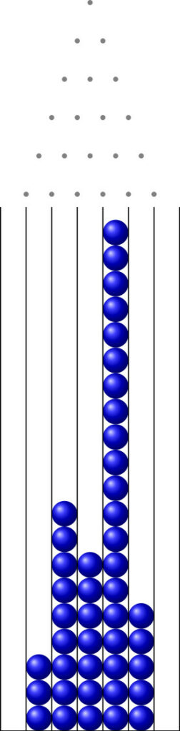
et j’obtiens le PDF suivant:

Mais à ce stade, si je ne fais rien de plus que compiler à nouveau, j’obtiens exactement le même document. Or, ce que je voudrais, c’est une autre simulation… Pour se faire, je suis obligé de supprimer le répertoire pythontex-files-temp créé lors de la compilation via pythontex.

Ce n’est pas pratique… C’est pour cela que je préfère la seconde façon.

Approche avec génération du code $\LaTeX$ en Python

Cette approche est à mon sens bien plus efficace.

On part du programme Python suivant:

from random import choice
from os import system

def simulation_galton(c = 7 , n = 20):
    base = c * [0]
    for bille in range(n):
        position = c // 2
        for clou in range(c-1):
            position += choice([-1,1])/2
            
        base[ int(position) ] += 1

    return base

def graph_latex( L ):
    ligne = '\\documentclass{standalone}\n'
    ligne += '\\usepackage{tikz}\n'
    ligne += '\\begin{document}\n'
    ligne += '\\begin{tikzpicture}\n'
    for i in range(len(L)): # pour chaque élément de L
        if L[i] != 0: # si l'élément est non nul
            for y in range(1,L[i]): # on trace L[i] billes à la verticale
                ligne += '\\shade[ball color = blue] (' + str(i+0.5) + ' , ' + str(y) + ') circle (5mm);\n'
    
    ligne += '\\draw[very thick] (0,0.5) -- (' + str(len(L)) + ',0.5);\n'
    for x in range( len(L)+1 ):
        ligne += '\\draw[very thick] ('+str(x)+','+str(0.5)+') -- ('+str(x)+','+str( max(L) )+');\n'
    for y in range( len(L) ):
        for x in range( y ):
            ligne += '\\fill[gray] (' + str(1+3-y/2+x) + ',' + str(max(L) + 0.5 + 1.5*(len(L)-y-1)) + ') circle (1mm);\n'
    ligne += '\\end{tikzpicture}\n'
    ligne += '\\end{document}'
    return ligne

"""
création du fichier LaTeX
"""
latex = graph_latex( simulation_galton(n=50) )
fichier = open('galton.tex' , 'w', encoding = 'utf8')
fichier.write( latex )
fichier.close()

"""
compilation via pdflatex
"""

system('pdflatex galton.tex')
system('start galton.pdf')

Il va d’une part simuler une expérience (ici, avec 7 colonnes et 50 billes), générer le fichier $\LaTeX$, le compiler et afficher le PDF, comme celui-ci par exemple:

Il est alors aisé de modifier légèrement le programme Python pour générer autant d’expériences que souhaité.

"""
création des fichiers LaTeX & PDF
"""
ext = [ 'log' , 'tex' , 'aux' ]
for k in range(5):
    latex = graph_latex( simulation_galton(n=50) )
    fichier = open('galton-'+str(k+1)+'.tex' , 'w', encoding = 'utf8')
    fichier.write( latex )
    fichier.close()

    """
    compilation via pdflatex
    """

    system('pdflatex galton-'+str(k+1)+'.tex')
    for e in ext:
        system('erase galton-' + str(k+1) + '.' + e)

Ici, j’ai opté pour le fait de supprimer tous les fichiers qui ne servent à rien pour ne garder que les fichiers PDF.

À noter que je suis sous Windows 10; j’utilise donc la commande « erase ». Sous Linux et MacOS, il me semble que c’est la commande « rm <fichier.ext> ».

La simulation de ces expériences est au programme de spécialité mathématiques en Terminale. Cette dernière approche peut donc aider les enseignant·e·s à construire un cours avec illustrations.